Example Notebook for the tunneling Fermions
This Notebook is based on the following paper from the Jochim group. In these experiments two fermions of different spins are put into a single tweezer and then coupled to a second tweezer. The dynamics is then controlled by two competing effects. The interactions and the tunneling.
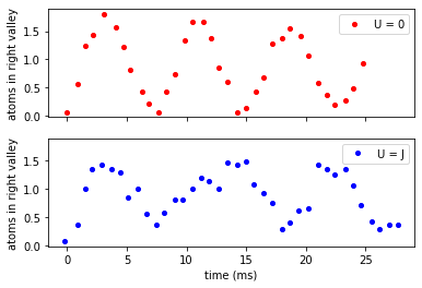
Let us first start by looking at the data, then look how the can be described in the Hamiltonian language and finally in the gate language.
import pennylane as qml
from pennylane import numpy as np
import matplotlib.pyplot as plt


import pandas as pd
data_murmann_no_int = pd.read_csv("Data/Murmann_No_Int.csv", names=["time", "nR"])
data_murmann_with_int = pd.read_csv("Data/Murmann_With_Int.csv", names=["time", "nR"])

# plt.figure(dpi=96)
f, (ax1, ax2) = plt.subplots(2, 1, sharex=True, sharey=True)
ax1.plot(
    data_murmann_no_int.time, data_murmann_no_int.nR, "ro", label="U = 0", markersize=4
)
ax2.plot(
    data_murmann_with_int.time,
    data_murmann_with_int.nR,
    "bo",
    label="U = J",
    markersize=4,
)
ax1.set_ylabel(r"atoms in right valley")
ax2.set_ylabel(r"atoms in right valley")
ax2.set_xlabel(r"time (ms)")
ax1.legend()
ax2.legend()
<matplotlib.legend.Legend at 0x1a9f421b6a0>
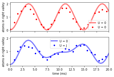
Analytical prediction
For the two atoms the Hamiltonian can be written down in the basis \(\{LL, LR, RL, RR\}\) as:
And we start out in the basis state \(|LL\rangle\). So we can write
from scipy.sparse.linalg import expm
J = np.pi * 134
# in units of hbar
U = 0.7 * J;
Nt_an = 50
t_analytical = np.linspace(0, 20, Nt_an) * 1e-3
H_With_Int = np.array([[U, -J, -J, 0], [-J, 0, 0, -J], [-J, 0, 0, -J], [0, -J, -J, U]])
H_Wo_Int = np.array([[0, -J, -J, 0], [-J, 0, 0, -J], [-J, 0, 0, -J], [0, -J, -J, 0]])
psi0 = np.zeros(4) * 1j
psi0[0] = 1.0 + 0j
print(psi0)
[1.+0.j 0.+0.j 0.+0.j 0.+0.j]
psis_wo_int = 1j * np.zeros((4, Nt_an))
psis_w_int = 1j * np.zeros((4, Nt_an))

for ii in np.arange(Nt_an):

    U_wo = expm(-1j * t_analytical[ii] * H_Wo_Int)
    psis_wo_int[:, ii] = np.dot(U_wo, psi0)

    U_w = expm(-1j * t_analytical[ii] * H_With_Int)
    psis_w_int[:, ii] = np.dot(U_w, psi0)

ps_wo = np.abs(psis_wo_int) ** 2
ps_w = np.abs(psis_w_int) ** 2
nR_wo = ps_wo[1, :] + ps_wo[2, :] + 2 * ps_wo[3, :]
nR_w = ps_w[1, :] + ps_w[2, :] + 2 * ps_w[3, :];
f, (ax1, ax2) = plt.subplots(2, 1, sharex=True, sharey=True)
ax1.plot(t_analytical * 1e3, nR_wo, "r-", label="U = 0", linewidth=4, alpha=0.5)
ax1.plot(
    data_murmann_no_int.time, data_murmann_no_int.nR, "ro", label="U = 0", markersize=4
)

ax2.plot(t_analytical * 1e3, nR_w, "b-", label="U = 0", linewidth=4, alpha=0.5)
ax2.plot(
    data_murmann_with_int.time,
    data_murmann_with_int.nR,
    "bo",
    label="U = J",
    markersize=4,
)
ax1.set_ylabel(r"atoms in right valley")
ax2.set_ylabel(r"atoms in right valley")
ax2.set_xlabel(r"time (ms)")
ax2.set_xlim(0, 20)
ax1.legend()
ax2.legend()
<matplotlib.legend.Legend at 0x1a9f4c05f40>
Pennylane
And now we also compare to the pennylane simulation. Make sure that you followed the necessary steps for obtaining the credentials as desribed in the introduction.
from pennylane_ls import *
from heroku_credentials import username, password
FermionDevice = qml.device("synqs.fs", shots=500, username=username, password=password)
In the experiments two Fermions are loaded onto the right side, i.e. into the wire 0 and 1.
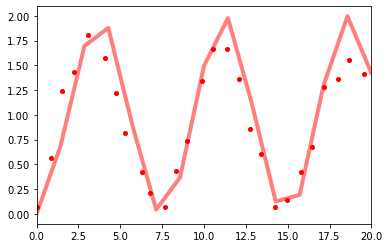
No interaction
In a first set of experiments there are no interactions and the two atoms are simply allowed to hop. The experiment is then described by the following very simple circuit.
@qml.qnode(FermionDevice)
def simple_hopping(theta=0):
    """
    The circuit that simulates the experiments.

    theta ... angle of the hopping
    """
    # load atoms
    FermionOps.Load(wires=0)
    FermionOps.Load(wires=1)

    # let them hop
    FermionOps.Hop(theta, wires=[0, 1, 2, 3])

    # measure the occupation on the right side
    obs = FermionOps.ParticleNumber([2, 3])
    return qml.expval(obs)
simple_hopping(0)
tensor([0., 0.], requires_grad=True)
print(simple_hopping.draw())
 0: ──Load──╭Hop(0)───┤
 1: ──Load──├Hop(0)───┤
 2: ────────├Hop(0)──╭┤ ⟨ParticleNumber⟩
 3: ────────╰Hop(0)──╰┤ ⟨ParticleNumber⟩
now let us simulate the time evolution
Ntimes = 15
times = np.linspace(0, 20, Ntimes) * 1e-3
means = np.zeros(Ntimes)
for i in range(Ntimes):
    if i % 10 == 0:
        print("step", i)
    # Calculate the resulting states after each rotation
    means[i] = sum(simple_hopping(-2 * J * times[i]))
step 0
step 10
and compare to the data
f, ax1 = plt.subplots(1, 1, sharex=True, sharey=True)
ax1.plot(times * 1e3, means, "r-", label="U = 0", linewidth=4, alpha=0.5)
ax1.plot(
    data_murmann_no_int.time, data_murmann_no_int.nR, "ro", label="U = 0", markersize=4
)
ax1.set_xlim(0, 20)
(0.0, 20.0)
Hopping with interactions
In a next step the atoms are interacting. The circuit description of the experiment is the application of the hopping gate and the interaction gate. It can be written as
@qml.qnode(FermionDevice)
def correlated_hopping(theta=0, gamma=0, Ntrott=15):
    """
    The circuit that simulates the experiments.

    theta ... angle of the hopping
    gamma ... angle of the interaction
    """
    # load atoms
    FermionOps.Load(wires=0)
    FermionOps.Load(wires=1)

    # let them hop
    # evolution under the Hamiltonian
    for ii in range(Ntrott):
        FermionOps.Hop(theta / Ntrott, wires=[0, 1, 2, 3])
        FermionOps.Inter(gamma / Ntrott, wires=[0, 1, 2, 3, 4, 5, 6, 7])

    # measure the occupation on the right side
    obs = FermionOps.ParticleNumber([2, 3])
    return qml.expval(obs)
Ntimes = 15
times = np.linspace(0, 20, Ntimes) * 1e-3
means_int = np.zeros(Ntimes)
for i in range(Ntimes):
    if i % 10 == 0:
        print("step", i)
    means_int[i] = sum(correlated_hopping(-2 * J * times[i], U * times[i]))
step 0
step 10
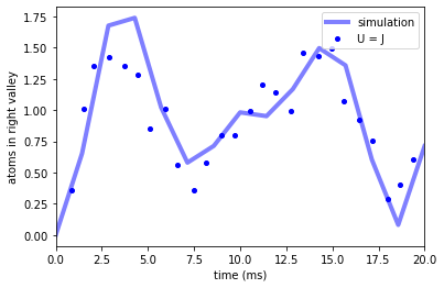
And we compare to the data to obtain
f, ax2 = plt.subplots(1, 1, sharex=True, sharey=True)

ax2.plot(times * 1e3, means_int, "b-", label="simulation", linewidth=4, alpha=0.5)
ax2.plot(
    data_murmann_with_int.time,
    data_murmann_with_int.nR,
    "bo",
    label="U = J",
    markersize=4,
)
ax2.set_ylabel(r"atoms in right valley")
ax2.set_xlabel(r"time (ms)")
ax2.legend()
ax2.set_xlim(0, 20)
(0.0, 20.0)
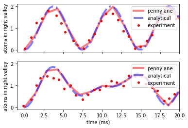
Summary
And finally we can compare the experimental data with all the descriptions.
f, (ax1, ax2) = plt.subplots(2, 1, sharex=True, sharey=True)


ax1.plot(times * 1e3, means, "r-", label="pennylane", linewidth=4, alpha=0.5)
ax1.plot(t_analytical * 1e3, nR_wo, "b-.", label="analytical", linewidth=4, alpha=0.5)
ax1.plot(
    data_murmann_no_int.time,
    data_murmann_no_int.nR,
    "ro",
    label="experiment",
    markersize=4,
)

ax2.plot(times * 1e3, means_int, "r-", label="pennylane", linewidth=4, alpha=0.5)
ax2.plot(t_analytical * 1e3, nR_w, "b-.", label="analytical", linewidth=4, alpha=0.5)
ax2.plot(
    data_murmann_with_int.time,
    data_murmann_with_int.nR,
    "ro",
    label="experiment",
    markersize=4,
)
ax1.set_ylabel(r"atoms in right valley")
ax2.set_ylabel(r"atoms in right valley")
ax2.set_xlabel(r"time (ms)")
ax1.legend(loc="upper right")
ax2.legend(loc="upper right")
ax1.set_xlim(-1, 20)
(-1.0, 20.0)