Propagation of a light pulse in a dispersive medium
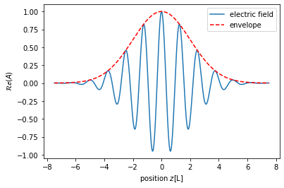
In this exercise we will solve the time evolution of a light pulse. We will describe its initial shape by function \(A(z,t = 0)\), which is assumed to be Gaussian for simplicity:
In plots etc, we will always only work with the real part of the wave package.
import numpy as np
import matplotlib.pyplot as plt
A quick initial plot.
# properties of the wave package
sigmaz = 2
k0 = 5

# parameters for plotting
Nz = 512
zmax = 7.5

zlin = np.linspace(-zmax, zmax, Nz)
Az = np.exp(-zlin**2/2/sigmaz**2)*np.exp(1j*k0*zlin)
Aenv = np.exp(-zlin**2/2/sigmaz**2)

f, ax = plt.subplots()
ax.plot(zlin, Az.real, label = 'electric field');
ax.plot(zlin, Aenv, 'r', ls = '--', label='envelope');
ax.set_xlabel('position $z$[L]');
ax.set_ylabel(' $\mathcal{Re}(A)$');
ax.legend()
<matplotlib.legend.Legend at 0x10f3a09a0>
We would now like to understand, how this wave-package propagates. In a non-linear medium the propagation is not easily solved, but we have to know the dispersion relationship of the medium. In our case, we will use the relationship:
For each single wavelength \(k\), we then know the time evolution of the wave package to be:
And the full time evolution is then obtain through the Fourier transform
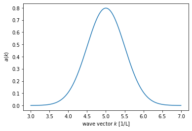
The intial wavepackage in Fourier space
As we know \(A(z,t=0)\), we can now also directly calculate:
This is a Gaussian integral of the type \(\int dz e^{-z^2} = \sqrt{\pi}\). We will rewrite:
We can now shift the limits of the integral to obtain:
Changing the variable of integration to \(z' = \frac{z}{\sqrt{2}\sigma}\), we end up with the integral:
It is Gaussian centered around \(k_c\) and of width \(\sigma_k = \frac{1}{\sigma}\)
Nk = 512;
klin = k0 + np.linspace(-4/sigmaz, 4/sigmaz, Nk);
ak = sigmaz/np.sqrt(2*np.pi)*np.exp(-sigmaz**2/2*(klin-k0)**2)

f, ax = plt.subplots()
ax.plot(klin, ak);
ax.set_xlabel('wave vector $k$ [1/L]');
ax.set_ylabel(' $a(k)$');
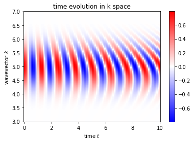
Time evolution in k space
We are now ready to simply calculate the time evolution of the wave package in k space. It is given by:
Quite importantly it remains a Gaussian in \(k\), but only we complex numbers. Ordering in polynoms of k, we have:
# parameters of the dispersion relation. You can set them freely
vp = 1
vg = 0.5
gamma = 1

#time
tmax = 10; Nt = 100;

tlin = np.linspace(0, tmax, Nt)
ks, ts = np.meshgrid(klin, tlin);

# the dispersion relationship
omegak = k0*vp+(ks-k0)*vg+gamma/2*(ks-k0)**2
aks = sigmaz/np.sqrt(2*np.pi)*np.exp(-sigmaz**2/2*(ks-k0)**2)

akt = ak*np.exp(-1j*omegak*ts);

f, ax = plt.subplots()
im1 = ax.pcolormesh(ts, ks, akt.real, cmap = 'bwr')
ax.set_xlabel('time $t$')
ax.set_ylabel('wavevector $k$')
ax.set_title('time evolution in k space')
f.colorbar(im1)
<matplotlib.colorbar.Colorbar at 0x10f620670>
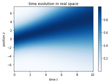
Time evolution in real space
We have now everything assembled together to calculate the time evolution in real space:
Given the nice form of \(a(k,t)\), we can already read it off:
The width will be the inverse of \(\sigma_x = \frac{1}{\sqrt{\sigma^2-i\Gamma t}}\)
It is centered around \(v_g t\)
It has some complicafted phase prefactor, which we will simply ignore here.
We then obtain:
To make it simpler to understand we rewrite:
The wave function has then the following form:
This is a Gaussian that is centered at \(z = v_gt\) with envelope:
zs, ts = np.meshgrid(zlin, tlin);

# the dispersion relationship
sigmat_sq = sigmaz**2+gamma**2*ts**2/sigmaz**2

azt = np.exp(-(zs-vg*ts)**2/2/sigmat_sq);

f, ax = plt.subplots()
im1 = ax.pcolormesh(ts, zs, azt, cmap = 'Blues')
ax.set_xlabel('time $t$')
ax.set_ylabel('position $z$')
ax.set_title('time evolution in real space')
f.colorbar(im1)
<matplotlib.colorbar.Colorbar at 0x10f6f4b20>